Introduction to Monte Carlo Tree Search
The subject of game AI generally begins with so-called perfect information games. These are turn-based games where the players have no information hidden from each other and there is no element of chance in the game mechanics (such as by rolling dice or drawing cards from a shuffled deck). Tic Tac Toe, Connect 4, Checkers, Reversi, Chess, and Go are all games of this type. Because everything in this type of game is fully determined, a tree can, in theory, be constructed that contains all possible outcomes, and a value assigned corresponding to a win or a loss for one of the players. Finding the best possible play, then, is a matter of doing a search on the tree, with the method of choice at each level alternating between picking the maximum value and picking the minimum value, matching the different players' conflicting goals, as the search proceeds down the tree. This algorithm is called Minimax.
The problem with Minimax, though, is that it can take an impractical amount of time to do a full search of the game tree. This is particularly true for games with a high branching factor, or high average number of available moves per turn. This is because the basic version of Minimax needs to search all of the nodes in the tree to find the optimal solution, and the number of nodes in the tree that must be checked grows exponentially with the branching factor. There are methods of mitigating this problem, such as searching only to a limited number of moves ahead (or ply) and then using an evaluation function to estimate the value of the position, or by pruning branches to be searched if they are unlikely to be worthwhile. Many of these techniques, though, require encoding domain knowledge about the game, which may be difficult to gather or formulate. And while such methods have produced Chess programs capable of defeating grandmasters, similar success in Go has been elusive, particularly for programs playing on the full 19x19 board.
However, there is a game AI technique that does do well for games with a high branching factor and has come to dominate the field of Go playing programs. It is easy to create a basic implementation of this algorithm that will give good results for games with a smaller branching factor, and relatively simple adaptations can build on it and improve it for games like Chess or Go. It can be configured to stop after any desired amount of time, with longer times resulting in stronger game play. Since it doesn't necessarily require game-specific knowledge, it can be used for general game playing. It may even be adaptable to games that incorporate randomness in the rules. This technique is called Monte Carlo Tree Search. In this article I will describe how MCTS works, specifically a variant called Upper Confidence bound applied to Trees (UCT), and then will show you how to build a basic implementation in Python.
Imagine, if you will, that you are faced with a row of slot machines, each with different payout probabilities and amounts. As a rational person (if you are going to play them at all), you would prefer to use a strategy that will allow you to maximize your net gain. But how can you do that? For whatever reason, there is no one nearby, so you can't watch someone else play for a while to gain information about which is the best machine. Clearly, your strategy is going to have to balance playing all of the machines to gather that information yourself, with concentrating your plays on the observed best machine. One strategy, called UCB1, does this by constructing statistical confidence intervals for each machine
where:
- \(\bar{x}_i\): the mean payout for machine \(i\)
- \(n_i\): the number of plays of machine \(i\)
- \(n\): the total number of plays
Then, your strategy is to pick the machine with the highest upper bound each time. As you do so, the observed mean value for that machine will shift and its confidence interval will become narrower, but all of the other machines' intervals will widen. Eventually, one of the other machines will have an upper bound that exceeds that of your current one, and you will switch to that one. This strategy has the property that your regret, the difference between what you would have won by playing solely on the actual best slot machine and your expected winnings under the strategy that you do use, grows only as \(\mathcal{O}(\ln n)\). This is the same big-O growth rate as the theoretical best for this problem (referred to as the multi-armed bandit problem), and has the additional benefit of being easy to calculate.
And here's how Monte Carlo comes in. In a standard Monte Carlo process, a large number of random simulations are run, in this case, from the board position that you want to find the best move for. Statistics are kept for each possible move from this starting state, and then the move with the best overall results is returned. The downside to this method, though, is that for any given turn in the simulation, there may be many possible moves, but only one or two that are good. If a random move is chosen each turn, it becomes extremely unlikely that the simulation will hit upon the best path forward. So, UCT has been proposed as an enhancement. The idea is this: any given board position can be considered a multi-armed bandit problem, if statistics are available for all of the positions that are only one move away. So instead of doing many purely random simulations, UCT works by doing many multi-phase playouts.
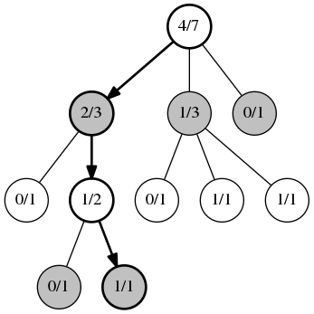
Selection
The first phase, selection, lasts while you have the statistics necessary to treat each position you reach as a multi-armed bandit problem. The move to use, then, would be chosen by the UCB1 algorithm instead of randomly, and applied to obtain the next position to be considered. Selection would then proceed until you reach a position where not all of the child positions have statistics recorded.
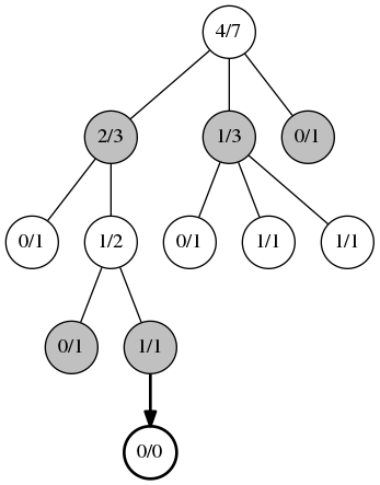
Expansion
The second phase, expansion, occurs when you can no longer apply UCB1. An unvisited child position is randomly chosen, and a new record node is added to the tree of statistics.
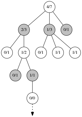
Simulation
After expansion occurs, the remainder of the playout is in phase 3, simulation. This is done as a typical Monte Carlo simulation, either purely random or with some simple weighting heuristics if a light playout is desired, or by using some computationally expensive heuristics and evaluations for a heavy playout. For games with a lower branching factor, a light playout can give good results.
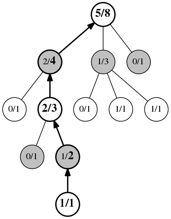
Back-Propagation
Finally, the fourth phase is the update or back-propagation phase. This occurs when the playout reaches the end of the game. All of the positions visited during this playout have their play count incremented, and if the player for that position won the playout, the win count is also incremented.
This algorithm may be configured to stop after any desired length of time, or on some other condition. As more and more playouts are run, the tree of statistics grows in memory and the move that will finally be chosen will converge towards the actual optimal play, though that may take a very long time, depending on the game.
For more details about the mathematics of UCB1 and UCT, see Finite-time Analysis of the Multiarmed Bandit Problem and Bandit based Monte-Carlo Planning.
Now let's see some code. To separate concerns, we're going to need a Board class, whose purpose is to encapsulate the rules of a game and which will care nothing about the AI, and a MonteCarlo class, which will only care about the AI algorithm and will query into the Board object in order to obtain information about the game. Let's assume a Board class supporting this interface:
class Board(object):
    def start(self):
        # Returns a representation of the starting state of the game.
        pass

    def current_player(self, state):
        # Takes the game state and returns the current player's
        # number.
        pass

    def next_state(self, state, play):
        # Takes the game state, and the move to be applied.
        # Returns the new game state.
        pass

    def legal_plays(self, state_history):
        # Takes a sequence of game states representing the full
        # game history, and returns the full list of moves that
        # are legal plays for the current player.
        pass

    def winner(self, state_history):
        # Takes a sequence of game states representing the full
        # game history.  If the game is now won, return the player
        # number.  If the game is still ongoing, return zero.  If
        # the game is tied, return a different distinct value, e.g. -1.
        pass
For the purposes of this article I'm not going to flesh this part out any further, but for example code you can find one of my implementations on github. However, it is important to note that we will require that the state data structure is hashable and equivalent states hash to the same value. I personally use flat tuples as my state data structures.
The AI class we will be constructing will support this interface:
class MonteCarlo(object):
    def __init__(self, board, **kwargs):
        # Takes an instance of a Board and optionally some keyword
        # arguments.  Initializes the list of game states and the
        # statistics tables.
        pass

    def update(self, state):
        # Takes a game state, and appends it to the history.
        pass

    def get_play(self):
        # Causes the AI to calculate the best move from the
        # current game state and return it.
        pass

    def run_simulation(self):
        # Plays out a "random" game from the current position,
        # then updates the statistics tables with the result.
        pass
Let's begin with the initialization and bookkeeping. The board object is what the AI will be using to obtain information about where the game is going and what the AI is allowed to do, so we need to store it. Additionally, we need to keep track of the state data as we get it.
class MonteCarlo(object):
    def __init__(self, board, **kwargs):
        self.board = board
        self.states = []

    def update(self, state):
        self.states.append(state)
The UCT algorithm relies on playing out multiple games from the current state, so let's add that next.
import datetime

class MonteCarlo(object):
    def __init__(self, board, **kwargs):
        # ...
        seconds = kwargs.get('time', 30)
        self.calculation_time = datetime.timedelta(seconds=seconds)

    # ...

    def get_play(self):
        begin = datetime.datetime.utcnow()
        while datetime.datetime.utcnow() - begin < self.calculation_time:
            self.run_simulation()
Here we've defined a configuration option for the amount of time to spend on a calculation, and get_play will repeatedly call run_simulation until that amount of time has passed. This code won't do anything particularly useful yet, because we still haven't defined run_simulation, so let's do that now.
# ...
from random import choice

class MonteCarlo(object):
    def __init__(self, board, **kwargs):
        # ...
        self.max_moves = kwargs.get('max_moves', 100)

    # ...

    def run_simulation(self):
        states_copy = self.states[:]
        state = states_copy[-1]

        for t in xrange(self.max_moves):
            legal = self.board.legal_plays(states_copy)

            play = choice(legal)
            state = self.board.next_state(state, play)
            states_copy.append(state)

            winner = self.board.winner(states_copy)
            if winner:
                break
This adds the beginnings of the run_simulation method, which either selects a move using UCB1 or chooses a random move from the set of legal moves each turn until the end of the game. We have also introduced a configuration option for limiting the number of moves forward that the AI will play.
You may notice at this point that we are making a copy of self.states and adding new states to it, instead of adding directly to self.states. This is because self.states is the authoritative record of what has happened so far in the game, and we don't want to mess it up with these speculative moves from the simulations.
Now we need to start keeping statistics on the game states that the AI hits during each run of run_simulation. The AI should pick the first unknown game state it reaches to add to the tables.
class MonteCarlo(object):
    def __init__(self, board, **kwargs):
        # ...
        self.wins = {}
        self.plays = {}

    # ...

    def run_simulation(self):
        visited_states = set()
        states_copy = self.states[:]
        state = states_copy[-1]
        player = self.board.current_player(state)

        expand = True
        for t in xrange(self.max_moves):
            legal = self.board.legal_plays(states_copy)

            play = choice(legal)
            state = self.board.next_state(state, play)
            states_copy.append(state)

            # `player` here and below refers to the player
            # who moved into that particular state.
            if expand and (player, state) not in self.plays:
                expand = False
                self.plays[(player, state)] = 0
                self.wins[(player, state)] = 0

            visited_states.add((player, state))

            player = self.board.current_player(state)
            winner = self.board.winner(states_copy)
            if winner:
                break

        for player, state in visited_states:
            if (player, state) not in self.plays:
                continue
            self.plays[(player, state)] += 1
            if player == winner:
                self.wins[(player, state)] += 1
Here we've added two dictionaries to the AI, wins and plays, which will contain the counts for every game state that is being tracked. The run_simulation method now checks to see if the current state is the first new one it has encountered this call, and, if not, adds the state to both plays and wins, setting both values to zero. This method also adds every game state that it goes through to a set, and at the end updates plays and wins with those states in the set that are in the plays and wins dicts. We are now ready to base the AI's final decision on these statistics.
from __future__ import division
# ...

class MonteCarlo(object):
    # ...

    def get_play(self):
        self.max_depth = 0
        state = self.states[-1]
        player = self.board.current_player(state)
        legal = self.board.legal_plays(self.states[:])

        # Bail out early if there is no real choice to be made.
        if not legal:
            return
        if len(legal) == 1:
            return legal[0]

        games = 0
        begin = datetime.datetime.utcnow()
        while datetime.datetime.utcnow() - begin < self.calculation_time:
            self.run_simulation()
            games += 1

        moves_states = [(p, self.board.next_state(state, p)) for p in legal]

        # Display the number of calls of `run_simulation` and the
        # time elapsed.
        print games, datetime.datetime.utcnow() - begin

        # Pick the move with the highest percentage of wins.
        percent_wins, move = max(
            (self.wins.get((player, S), 0) /
             self.plays.get((player, S), 1),
             p)
            for p, S in moves_states
        )

        # Display the stats for each possible play.
        for x in sorted(
            ((100 * self.wins.get((player, S), 0) /
              self.plays.get((player, S), 1),
              self.wins.get((player, S), 0),
              self.plays.get((player, S), 0), p)
             for p, S in moves_states),
            reverse=True
        ):
            print "{3}: {0:.2f}% ({1} / {2})".format(*x)

        print "Maximum depth searched:", self.max_depth

        return move
We have added three things in this step. First, we allow get_play to return early if there are no choices or only one choice to make. Next, we've added output of some debugging information, including the statistics for the possible moves this turn and an attribute that will keep track of the maximum depth searched in the selection phase of the playouts. Finally, we've added code that picks out the move with the highest win percentage out of the possible moves, and returns it.
But we are not quite finished yet. Currently, our AI is using pure randomness for its playouts. We need to implement UCB1 for positions where the legal plays are all in the stats tables, so the next trial play is based on that information.
# ...
from math import log, sqrt

class MonteCarlo(object):
    def __init__(self, board, **kwargs):
        # ...
        self.C = kwargs.get('C', 1.4)

    # ...

    def run_simulation(self):
        # A bit of an optimization here, so we have a local
        # variable lookup instead of an attribute access each loop.
        plays, wins = self.plays, self.wins

        visited_states = set()
        states_copy = self.states[:]
        state = states_copy[-1]
        player = self.board.current_player(state)

        expand = True
        for t in xrange(1, self.max_moves + 1):
            legal = self.board.legal_plays(states_copy)
            moves_states = [(p, self.board.next_state(state, p)) for p in legal]

            if all(plays.get((player, S)) for p, S in moves_states):
                # If we have stats on all of the legal moves here, use them.
                log_total = log(
                    sum(plays[(player, S)] for p, S in moves_states))
                value, move, state = max(
                    ((wins[(player, S)] / plays[(player, S)]) +
                     self.C * sqrt(log_total / plays[(player, S)]), p, S)
                    for p, S in moves_states
                )
            else:
                # Otherwise, just make an arbitrary decision.
                move, state = choice(moves_states)

            states_copy.append(state)

            # `player` here and below refers to the player
            # who moved into that particular state.
            if expand and (player, state) not in plays:
                expand = False
                plays[(player, state)] = 0
                wins[(player, state)] = 0
                if t > self.max_depth:
                    self.max_depth = t

            visited_states.add((player, state))

            player = self.board.current_player(state)
            winner = self.board.winner(states_copy)
            if winner:
                break

        for player, state in visited_states:
            if (player, state) not in plays:
                continue
            plays[(player, state)] += 1
            if player == winner:
                wins[(player, state)] += 1
The main addition here is the check to see if all of the results of the legal moves are in the plays dictionary. If they aren't available, it defaults to the original random choice. But if the statistics are all available, the move with the highest value according to the confidence interval formula is chosen. This formula adds together two parts. The first part is just the win ratio, but the second part is a term that grows slowly as a particular move remains neglected. Eventually, if a node with a poor win rate is neglected long enough, it will begin to be chosen again. This term can be tweaked using the configuration parameter C added to __init__ above. Larger values of C will encourage more exploration of the possibilities, and smaller values will cause the AI to prefer concentrating on known good moves. Also note that the self.max_depth attribute from the previous code block is now updated when a new node is added and its depth exceeds the previous self.max_depth.
So there we have it. If there are no mistakes, you should now have an AI that will make reasonable decisions for a variety of board games. I've left a suitable implementation of Board as an exercise for the reader, but one thing I've left out here is a way of actually allowing a user to play against the AI. A toy framework for this can be found at jbradberry/boardgame-socketserver and jbradberry/boardgame-socketplayer.
This version that we've just built uses light playouts. Next time, we'll explore improving our AI by using heavy playouts, by training some evaluation functions using machine learning techniques and hooking in the results.
Note
UPDATE: The diagrams have been corrected to more accurately reflect the possible node values.
Note
UPDATE: Achievement Unlocked! This article has been republished in Hacker Monthly, Issue 66, November 2015.